ForSys Overview

ForSysX was developed by the US Forest Service, Rocky Mountain Research Station to provide a platform for prioritizing risk reduction and restoration investments using spatial optimization methods that are widely used in conservation planning and the forest industry.  The development of ForSys was motivated by gaps in decision support tools for rendering the growing number of Forest Service land condition assessments into optimized projects areas as part of prioritization and planning efforts. ForSys is designed around the concept that restoration and risk reduction activities occur at the stand polygon scale (1-20 ha; 2.5 – 50 acres) that need to be organized into project areas (5,000 – 25,000 acres) to achieve landscape scale management goals and meet logistical and administrative constraints. ForSys solves typical spatial planning problems where treatments are allocated to optimize one or more restoration objectives accounting for multiple hierarchical spatial constraints and treatment thresholds. ForSys integrates forest landscape planning, spatial optimization, and the science and literature on scenario analysis that emphasizes the importance of examining large arrays of management scenarios and considering uncertain future disturbance. The ForSysX interface was developed with an emphasis for wide application by non-technical user and employs a spatial optimization algorithm that can be easily explained to stakeholders and compared to opaque mathematical programming approaches. ForSysX has been applied to prioritization projects at a range of scales, including sub-watershed projects, national forests, regions, and the entire national forest network.

This Quick Start Guide was designed to illustrate  the program’s basic functionality, familiarize the user with inputs and results using a simple example ForSysX run, and provide data descriptions and preparation recommendations for users who wish to use local datasets within the program. Note that the ForSys platform currently exists in three formats: 1) an executable C++ desktop application (ForSysX) described here, 2) an R script (ForSysR) available for R programmers via github, and 3) a DLL created from the C++ program that can be wrapped within other applications. This manual covers only ForSysX using the tutorial dataset as described at the end of this document (section 6).

1. ForSysX Interface

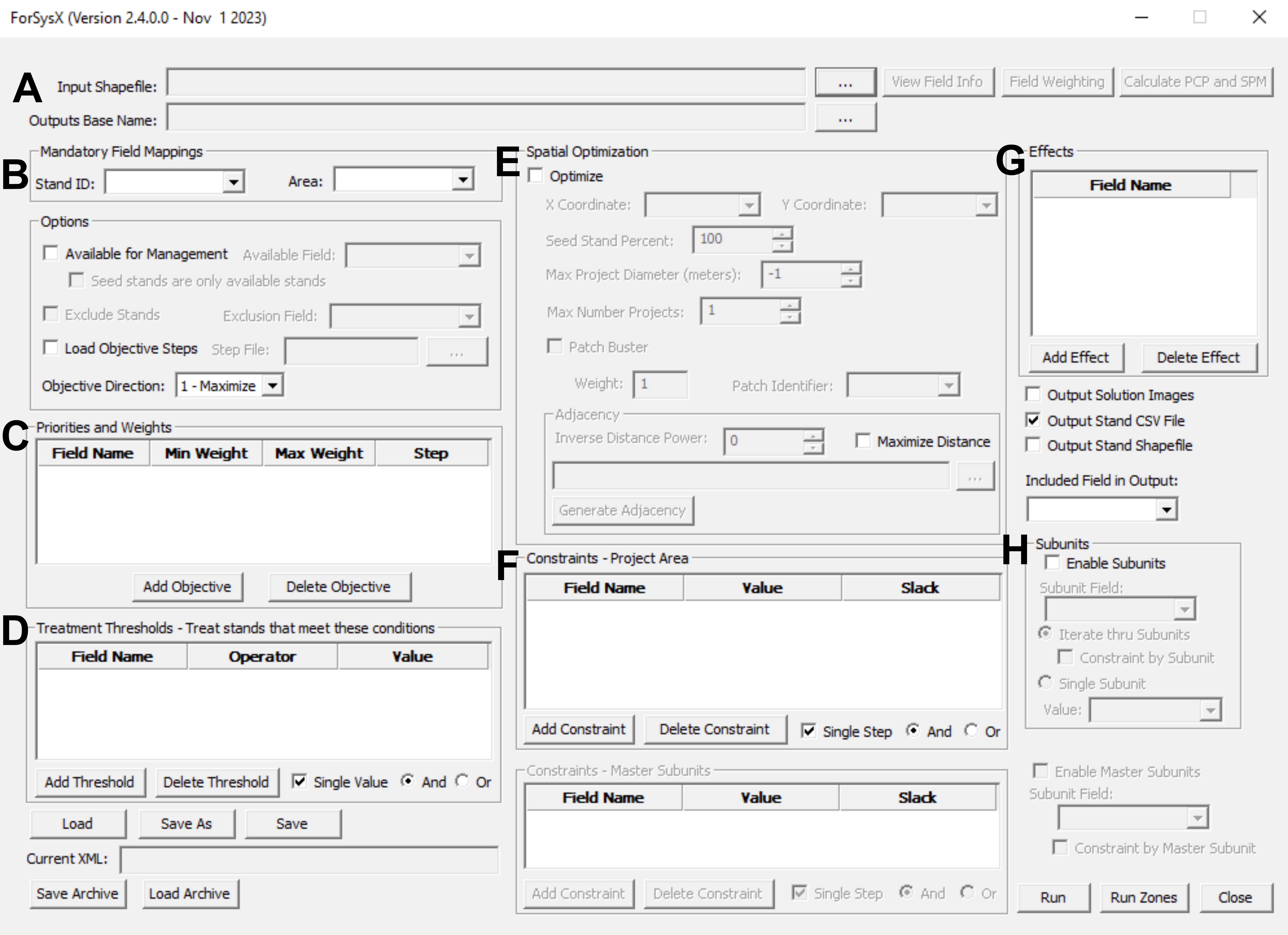
The ForSysX interface is divided into eight panels and associated user defined inputs required for simulating scenarios: a) specify input shapefile, b) assign data field names, c) select priorities and weights, d) specify treatment thresholds, e) select optimization options, f) select treatment constraints, g) specify treatment effects and output settings, and h) identify landscape subunits (pre-defined planning areas) if present, and identify subunit-specific constraints for nested runs (Fig. 1). The primary input to ForSys is a GIS shapefile that contains stand-scale including treatment thresholds, constraints and management subareas, if present. The priority and weights panel provides functionality to input multiple treatment priorities and associated weight ranges that instruct ForSys to iterate through all combinations of objectives and weights with increments specified in the Step field. Treatment thresholds specify the stand scale conditions that must be met to make a stand available for treatment. Constraints are entered to control the activity (e.g., area treated) at the project scale.

1.A. Input data

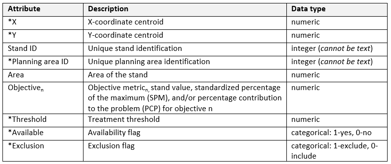
including a unique identification code and total stand area. The shapefile also contains fields describing the characteristics of each stand with respect to the objective, treatment threshold, stand availability, investment or activity constraint, and pre-defined planning area and other subdivisions, such as national forest (Table 1). The Outputs Base Name dialogue box near the top of the screen includes the user-defined name for the output files as well as the directory to which outputs will be saved. After uploading the shapefile, the user can confirm that it was read correctly by selecting the View Field Info option. If the Optimize option is used the shapefile must include an X and Y location field and the user must generate the required adjacency file using the Generate Adjacency option and then specify that file with the Use Adjacency option.

To normalize objective metrics to create a standardized reporting metric or to prioritize objectives of varying units and scales, the user can select Calculate PCP and SPM (Fig. 2). This option calculates the ‘percentage contribution to the problem’ (PCP) for each selected metric such that the stand is assigned the percentage value it contributes to the entire landscape. This option also calculates the ‘standardized percentage of the maximum’ (SPM) for each selected metric such that the stand is assigned the percentage value of the maximum across the entire landscape.  Weighting multiple priorities based on the SPM value will reduce the potential bias of a metric with higher values. Both the PCP and SPM calculations can be set to be calculated only on the available landscape as determined in section 1.B. The user must select an available field prior to calculating PCP and SPM if these metrics should only be calculated on the available landscape. Note that it is important to consider stand size in these calculations, otherwise stand selection will be biased towards larger stands. For datasets where there is a large range in stand size, metrics should be weighted to account for size. The Calculate PCP and SPM function has the option to Multiply by area of stand to automatically account for stand size in calculation (Fig. 2).

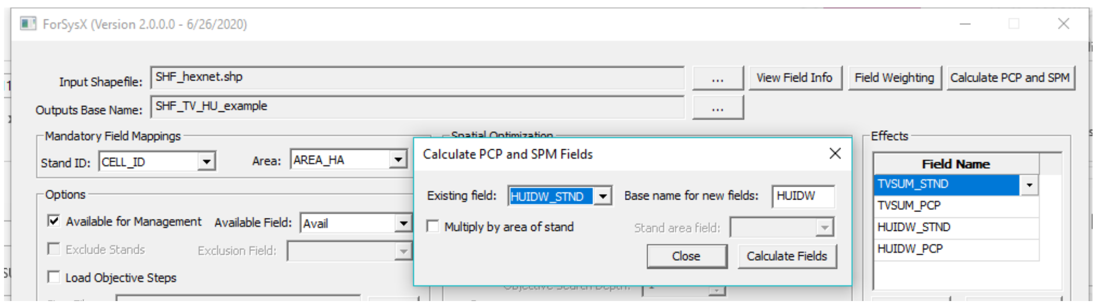
To normalize objective metrics among stands of varying size or create a standardized reporting metric to compare objectives of varying units, the user can select Calculate PCP and SPM (Fig. 2).  This option calculates the ‘percentage contribution to the problem’ (PCP) for each selected metric such that the stand is assigned the percentage value it contributes to the entire landscape.  This option also calculates the ‘standardized percentage of the maximum’ (SPM) for each selected metric such that the stand is assigned the percentage value of the maximum across the entire landscape.  Weighting priorities based on the SPM value will reduce the potential bias of large stands.  Both the PCP and SPM calculations can be set to be calculated only on the available landscape as determined in section 1.B. The user must select an available field prior to calculating PCP and SPM if these metrics should only be calculated on the available landscape. The SPM metric is used to account for varying stand sizes when weighting objectives.

Table 1. Basic content of the input shapefile attribute table. Treatment thresholds may include expected wildfire behavior, timber volume, or other operational restrictions that must be met to trigger treatment within a stand. Simple treatment restrictions can also be integrated as a treatment availability flag (e.g., a field in which manageable = 1, non-manageable = 0 could be used to include only manageable areas). The user can employ stand-level “percent contribution to the problem” (PCP) objective metrics to homogenize units among the different objectives and facilitate output analysis and interpretation (see section 1.A). Some attributes (*) are optional depending on the selection method being used.

1.B. Mandatory field mappings

A user must define a numeric stand ID field and stand area metric.  ForSysX allows users to indicate if all stands are available for treatment using the Available Field which is a binary field where 1 = available and 0 = unavailable, intended to prevent treatment in dispersed protected areas within the landscape. The user also selects whether ForSysX is maximizing or minimizing objectives (Objective Direction). The objective direction will depend on how treatment objectives are valued. Select the 1-Maximize option to optimize the objective total, and 0-Minimize to minimize the total objective. If the user is interested in running ForSysX for various objectives, all objective metrics should present the same direction logic (e.g., the highest priority for the highest values in all objective metrics). If this is not the case by default, the objective ramp should be inverted using GIS software before loading the input file.

1.C. Objective priorities and weights panel

ForSysX allows the user to consider multiple objectives and weights to prioritize stands for treatment. Multiple priorities are combined in an additive objective equation using the specified weights. The user must select Add Objective to identify the objective field name from the attribute table of the input data. Delete Objective removes the highlighted row. In multi-objective projects, the user must specify the Min Weight, Max Weight and Step as integer values. The steps represent the intervals between the maximum and minimum weight that determine the objective weight combinations. These values are filtered to exclude repetitive weights (e.g. weights 1-1 will provide the same results as weights 2-2 or 3-3 for a set of two-priority scenarios). For two objectives if a user selects weights between 0 and 3, ForSysX will run nine scenarios. Each scenario represents one combination of weights.  For example, if objective1 is weighted 0 and objective2 is weighted 3, ForSysX will prioritize stands with high values of objective2 and will not consider objective1. If both objective1 and objective2 are weighted 1, ForSysX will prioritize stands with high values of both objectives.  When using the spatial optimization feature, the program allows the user to select treatment Type including Both, Treat and Non-Treat.  Using Treat, only stands that are selected for treatment based on any threshold values will count towards the objective, while all stands within the patch are included using Both, whether or not the threshold is met by a stand. See note above about normalizing multiple objectives in section 1A.

1.D. Treatment thresholds panel

Treatment thresholds specify conditions that must be met in order for a stand to be considered for treatment. The user can remove this option by clicking on Delete Threshold. Available threshold operators include <, ≤, =, ≥, and >. For a single threshold the user must select the Field Name and Operator, and enter the threshold value.  If a user wants to step through multiple thresholds (adding more scenarios to the run), the user must set a Min Value and a Max Value. The Step option operates to explore the impact of a range of thresholds. Increasing the threshold on a variable may increase or decrease the number of stands available for treatment, depending on the operator in use. Multiple thresholds can be included, and the user can specify if they are and/or thresholds.

1.E. Optimization panel

The optimization panel (Fig. 1E) provides a wide range of spatial options for simulating scenarios. Users should test the optimization process using a small test area since many problems can take a long time to solve on large landscape. Basic functionality is as follows:

1. If the Optimize box is not checked and subunits are not used ForSys will simply sort the stands based on the objective values, treating those that meet the treatment thresholds, until the constraints are met. This solution is the absolute optimum given treatments can be located anywhere in the project area.

2. If the Optimize box is not checked and enable subunits (Fig. 1H) is checked then the process above will be executed for each subunit. Note that constraints can be specified for each subunit with a fixed value for all subunits, or a value read from the input shapefile, using the Constraint by Subunit option.  

3. If the Optimize box is checked then ForSys will spatially optimize projects by aggregating treatments using the heuristic. Stands are selected for treatment based on the objective value provided they meet the treatment threshold. Stands must be adjacent to be added to the project.

The following options and requirements are specifically for the Optimize option:

1. ForSysX can use a spatial aggregation function to cluster treatments into patches based on stand availability and priority values (versus pre-existing planning areas). This process is initialized by selecting the Optimize option. The procedure creates the user specified number of project areas sequentially, each having a lower total objective. The X and Y coordinate centroids must be identified in the input shapefile specified.

2. Max Project Diameter (meters) limits the maximum project diameter with the default of no maximum specified (-1).  Limiting the project diameter can substantially reduce processing times. Users can calculate an initial project diameter as Diameter = 2* sqrt(hectares/2.14) which assumes a circular project.

3. Seed Stand Percent. This option controls how many of the stands are used as seeds to build optimized projects. Using a lower number can result in lower objective values but faster processing time. Initial runs can use 10 to 15% to ensure that the problem is correctly formulated. This option is particularly useful for very large landscapes as a way to speed up processing time.

4. Max Number of Projects. The total number of projects requested from ForSysX should be specified as an integer value. If there is insufficient treatable area to create a project or if the constraints have not been met the Validity field in the output CSV file will indicate Invalid.

5. Generate Adjacency. Optimization requires an adjacency file created using the Generate Adjacency option is used to generate an adjacency matrix prior to the run. The adjacency constraint is used by the program to build more or less contiguous treatment patches based on the objective function while not exceeding the treatment constraint (see section 1.F).

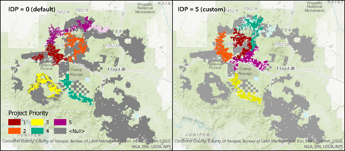
6. Inverse Distance Power (IDP) is used to control the compactness of a project by penalizing the heuristic for roaming far from the project centroid. The user can adjust the treatment aggregation pattern by changing the Inverse Distance Power (IDP) value (Fig. 3). Increasing the value will penalize stands farther away that might have a higher objective value and result in more or less circular, “clumpier” or tighter project patches with a higher density of treated stands within the optimized project.

7. Maximize Distance. This option will spread out projects such that each successive project is located in a way that maximizes distance between them.

Patch Buster is an experimental algorithm designed to address the problem where treatments are being used to optimally fragment large areas of continuous fuels that, for instance, will support crown fire behavior. Contact the authors for more information. When the Optimize option is not activated, ForSysX identifies the stands that maximize or minimize the objective function within the activity constraints, irrespective of spatial relationships within each project area.

1.F. Constraints panel

The constraints panel (Fig. 1F) controls treatment activity levels generally at the scale of the project. The most common constraint is the total treated area per project but can be expressed as a treatment budget or target amount of activity (e.g., harvest volume). Multiple constraints can be specified, and the optimization process will stop when the first constraint is met. Constraints can also be stepped to generate multiple scenarios at different levels of constraints by unchecking the Single Step option and specifying a minimum (Start Value) and maximum constraint value (Stop Value). The Step field indicates the designated interval ForSys will use to step through the min and max constraint values. It may be impossible, based on stand values, to meet a constraint precisely, so the user can specify a Slack interval. Any solution which falls within the constraint less the slack is considered valid in the results. ForSys will never exceed the constraint value. The outputs will include project-level summary statistics for each planning area or optimized project, including a Valid or Invalid flag, which indicates whether or not the solution is within the user-defined range. When the scenario contains subunits and the Constrained by Subunit option is invoked, the user can specify a field in the input shape file that contains the constraint level for each subunit (see section 1.H.).

1.G. Effects panel

The Effects panel provides options for different output files and variables included within them. The Add Effect button provides a way to specify values output into the CSV file which contains one record for each project (Fig. 1G); the Delete Effect will remove a selected value. For each field specified in the effects box the values will be summed at the scale of each project. Both total values and the value associated with just the treated stands are included as indicated by the headers in the output file. The ETrt prefix indicates the values of treated stands and the ESum prefix indicates the total of both treated and untreated stands that are considered available for treatment based on the Available Field. The Included Field in Output option simply echoes a single value from the input to the output and can be used to label project with administrative or other categorical values. See note in section 1A about normalizing values for reporting effects for objectives with variable units such as comparing timber volume with wildfire hazard.

1. The Output Solution Images option creates a map of projects for each scenario.

2. The Output Stand CSV File option generates a data table for stands selected for treatment in each project with the inputs and outputs for each weighted scenario. Note that the data in this CSV is identical to the shapefile output and can be joined to the input shapefile for mapping, rather than selecting the Output Stand Shapefile option described below.

3. The Output Stand Shapefile option generates a shapefile for stands selected for treatment in each project with the inputs and outputs for each weighted scenario. Note that generating a shapefile can significantly increase processing time.

1.H. Subunits panel

The subunit panel contains options to solve hierarchical planning problems. The Enable Subunits option must be checked and the Subunit Field set to the field that identifies the unique planning area ID. A user can choose to either create a static constraint for each planning area (e.g., treat 2000 ha/planning area) or create planning area-specific values by creating a constraint field (e.g., set constraints to 20% of each planning area). Constraint by Subunit allows the user to specify the planning area-specific constraint. Here the Field Name represents the field containing the value to be summed (e.g., hectares) and the Value Field represents the subunit-level constraint value field (e.g., Target_20percent contains the number of ha needed to treat 20% of the subunit area). The Single Subunit option allows a user to run the program for a single planning area to test the functionality of a scenario. In this case, the Value option must be selected to determine which planning area to process.

The Enable Master Subunits allows the user to add an additional scale of constraints above the subunits. For instance, subunits could be ranger districts and master subunits could be national forests for a region-wide scenario where each district and forest has unique constraints.

The Run Zones button allows the user to bundle multiple ForSys runs and execute them serially each having a different set of parameters.  Each individual ForSys run is set up and saved as an XML file, then the XML files are loaded using the Run Zones button and batch processed.  A single results CSV is generated containing the outputs for all runs where each run is appended after the last.

2. ForSysX Outputs

Multiple types of output files can be generated with each run: 1) a summary text file of input parameters, project level summary statistics for results, and the run duration (*_Summary.txt); 2) a stand table for each weighted solution, which includes data on every stand selected for treatment; 3) a table with input parameters, summary statistics (ESum_*) and treatment effects (“ETrt_*”) for all the objective weighting combinations combined (*_Results.csv); 4) a shapefile (*.shp) with an attribute table that identifies the planning area o project area locations (ProjectNumber field), input parameters, and stands selected for treatments (Treat = 1 for the treated units, and Treat = 0 for untreated units within the project corresponding to non-manageable areas and stands that do not meet the thresholds); and 5) output solution images (*.jpg) for every scenario where the user can quickly check the treatment allocation without opening the shapefile. The Summary and Result files are output for every run, but stand-level outputs, shapefiles, and image files must be specifically included (or excluded) by making selections under the Effects panel. The program will run faster if shapefiles are not included in the output. Stand .csv files can always be joined back to the original stand shapefile. ForSysX will notify a user if files should be appended or overwritten for output files with identical names.

3. Saving Runs

The user can save the run settings in a file (*.xml) using the Save or Save As functions or the whole analysis including settings and input data in a compressed file package (*.ltd) with Save Archive. For the former, only pathways and settings will be saved, so if files are moved the xml will not load properly. File pathways can be edited within a text editor when sharing xml files across users. The compressed package, on the other hand will contain the input shapefile (*.shp), adjacency file (*.csv), and prioritization parameter or settings (*.xml file) and does not require edits to open and run. Simply open the interface and select Load Archive. All inputs are decompressed into a user-defined folder location when opening the package.

4. Data preparation and structure

ForSysX input data are stored in a GIS shapefile attribute table. The variables described in this section are used to populate the fields described in section 1.A. There are five primary types of stand data included in the table for most ForSysX runs: 1) land base variables, 2) exclusion variables, 3) priority or objective variables, 4) contribution variables, and 5) target variables. See “Creating a Custom Dataset for ForSysX” for more details on creating a custom dataset.

4.A. Land base variables

For Forest Service datasets, stands generally include administrative attributes (examples in parentheses are variables in the tutorial dataset): a unique stand identifier (Cell_ID), pre-defined planning area identifier (PA_ID) if available, national forest (FORESTNAME or FORESTID), and region (Region). Other subunit delineations such as PODS, ownership, etc can be included and used to partition or constrain the problem.

4.B. Exclusions

The exclusion option is meant to exclude large areas for treatment that are within the landscape that were retained for convenience for mapping outputs.  For instance, wilderness and roadless areas can be included in the input shapefile so that the outputs display an entire national forest for convenience.  This is in contrast to the Available for Management option which is intended to prevent treatments within the study area on small, dispersed stands that are restricted for management based on forest plans (e.g., riparian areas, old growth).

4.C. Priority/value variables

Priority variables describe management objectives and can include a wide range of quantitative metrics including stand density index, building exposure from wildfire, wildfire hazard, wildfire risk to drinking water, ecological departure,  biodiversity, carbon, for example. ForSysX uses these metrics, singularly or in weighted combinations to build optimized project areas while adhering to constraints and treatment thresholds. The priorities can be used as raw values or converted to a standardized percent of the maximum (SPM) (described in section 1.A) to reduce scaling issues in multi-objective simulations. The SPM value is calculated as the percent of the maximum value for each priority.  A “percent contribution to the problem” (PCP) value can also be calculated to help interpret outcomes from treatments across different priority variables. The PCP is calculated as the percent of the sum of all stand values for a given priority. In some cases the meaning of the PCP is clear, for example the total percent of building exposure that is treated for a given scenario or a given planning area. For priorities that are based on an index or non-market value, describing this output is more challenging. Treating X% of the wildfire hazard potential, for example, may be less meaningful than an analysis of the pre- and post-treatment expected flame length of treated stands. Managers who wish to include new local priorities should consider how to understand the progress being made towards key performance indicators. But PCP values do allow users to compare attainment across multiple priorities such as wildfire risk to biodiversity versus buildings etc. As noted in section 1A it is important to incorporate stand size into these metrics for datasets where stand size varies considerably.

4.D. Determining suitability of data for use in ForSysX

The resolution and extent of spatial data must meet certain criteria for use in ForSysX. Data that are intended for use as priority variables must be at a higher resolution than the planning area scale, and ideally a higher resolution than the average stand size. Data intended for use as stand exclusion variables have no restrictions to their resolution, as they act as a filter. Past work has shown that very large variability in stand size can bias results since area is generally correlated with total objective. As a rough guide, stands ranging in size from 1 to 100 acres have functioned well in the program, although area weighting the values will correct for differences in most cases.  Data included in the model must align with management objectives and questions; and scenarios including priorities, constraints and treatment thresholds must be well developed prior to developing a final dataset for input into ForSysX.

4.E. Data preparation

There are five steps to preparing data for inclusion in ForSysX scenarios recognizing that it is import to first identify key objectives and management questions and how to use quantitative metrics to address these questions: 1) determine what dataset will be used as a stand layer, 2) identify the type of data you are adding, 3) determine how to attribute the data to the stand layer depending on data type, 4) spatially link data with stands using tools such as the ArcGIS tool Zonal Stats as Table, and 5) join the zonal statistic output data to the stand attribute table.  Stand layers can be obtained from FSVEG and populated with attributes with FSVEG-Spatial. Stand polygons or grids are intersected with land base variables such as ownership, forest plan land designations, Districts, Forests, etc.  ForSysX requires certain variables to have specific data types (see Table 1) and cannot contain null values. Users need to examine maps of each priority variable and summary statistics prior to running scenarios to understand how the values are distributed across the landscape. For instance, two priorities that are spatially correlated will not generate significantly different priority project areas.  See also the QuickStart_CreateACustom_ForSysX_2.0_Dataset.pdf quick start guide.

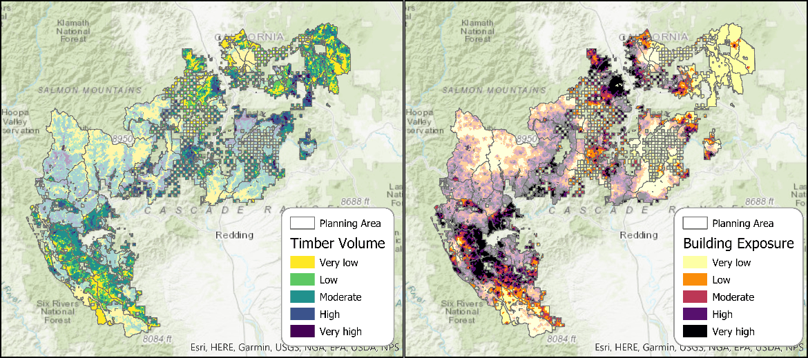
5. Example ForSysX Application on the Shasta-Trinity National Forest

In this first example we present a simple two-priority tradeoff analysis in which stand selections occur within pre-defined planning areas on the Shasta-Trinity National Forest. Stands are prioritized to either maximize harvest volume versus treating areas to reduce building exposure from wildfires ignited on the national forest. The study area is approximately 875,000 ha and is comprised of 41 pre-defined planning areas (Fig. 4) ranging in size from 845 to 15,000 treatable hectares. Stands are based on a regular hexnet grid intersected by ownership boundaries. There is a total of n = 22,408 treatment units or stands ranging in size from 5 to 61 ha. Wilderness areas, water bodies, and other protected areas or stands that are not available for mechanical treatment were excluded in scenarios, resulting in 351,243 ha of treatable area.

6. GettingStarted with ForSysX

The following section describes how to install ForSysX,load and run an example ForSysX scenario, explore the outputs that ForSysXproduces, and provide interpretation of the outputs.

6.A. Step-by-step instructions:

1. Request ForSysX and the associated archives (See Get Started):

   o ForSysX package which includes the program and associated libraries

   o ForSysX tutorial data for the Shasta-Trinity National Forest study area (ForSysX_Shasta_Tutorial.zip)

   o ForSysX Excel graphing program described in section 6.D is also available (ForSysXOutputGraphs_2019-11-20.zip)

2. Create a folder to store the program and data. Move zip files to that folder and extract their contents to the folder.

3. Open the ForSysX.exe program and select the Load Archive option at the bottom right panel.

4. Navigate to the folder you created above and open STF_predefined_example.ltd. The .ltd file is a zipped archive, so ForSysX will ask where you want to put the files. Save the files into the directory of your choice when prompted. This will be your root directory for ForSysX scenario outputs. Your ForSys program should now look like the screenshot in Fig. 5.

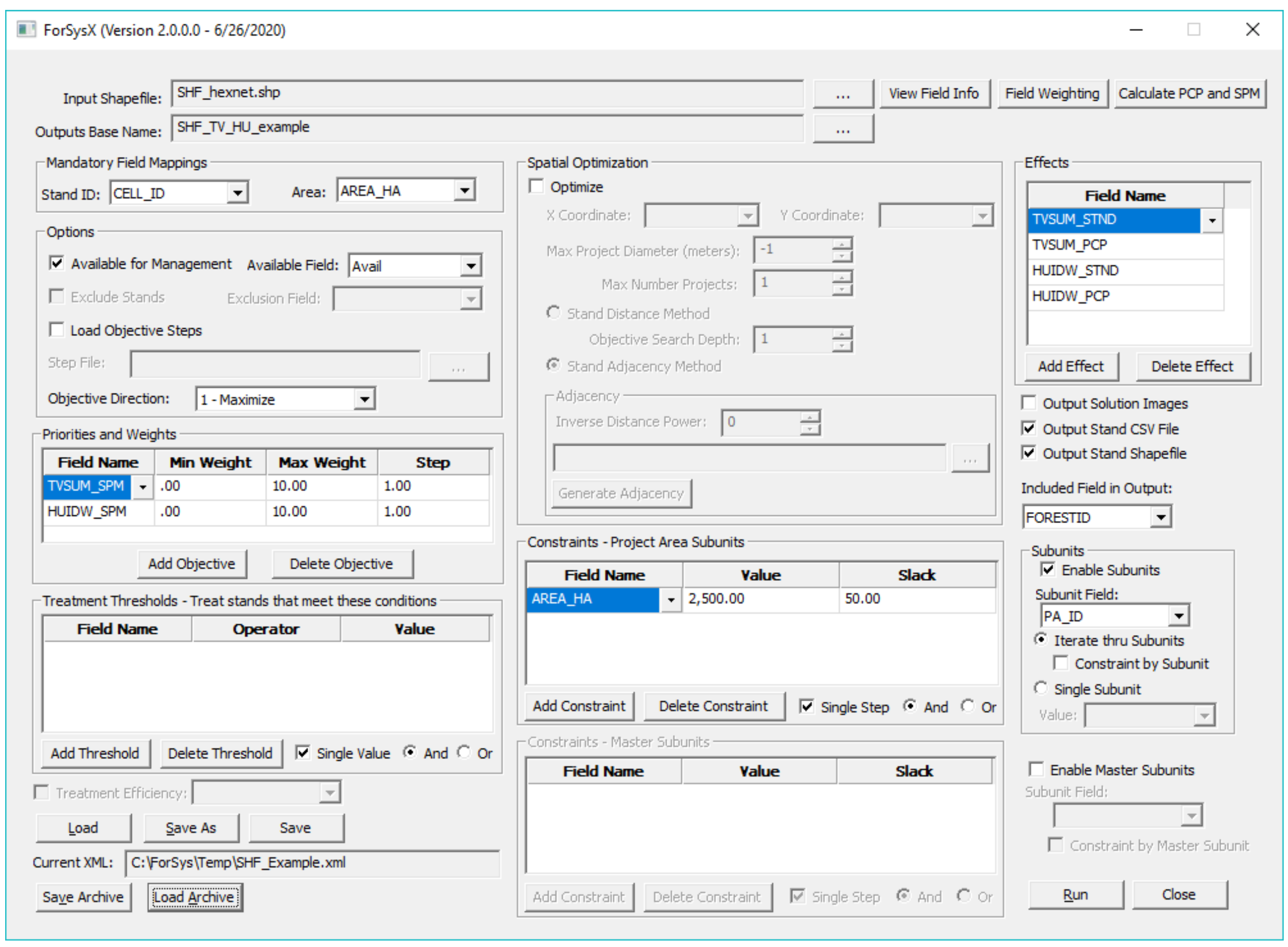
5.     Interpreting the example ForSysX scenario. This example analysis from the Shasta-Trinity National Forest explores tradeoffs between harvest volume and building exposure from wildfires ignited on national forest stands that spread to communities. The tradeoff is quantified by simulating a range of relative weights between the two priorities and examining the resulting objective values in the outputs. Note that if you hover over any ForSysX setting, popup text will describe the setting. In this analysis, stands available for treatment are set by the Available Field, which in this case describes whether active management is permitted. Next, the analysis will look at priority metrics for TVSUM_SPM and HUIDW_SPM with weighting combinations ranging from 0 to 10 in 1 increment steps. No treatment thresholds are defined, meaning all manageable stands (designated with the Available Field) will be considered. The analysis constrains treatments to 2,500 hectares for each of the 41 planning areas with a 50-ha slack (ForSysX will consider the result valid if it can treat up to 2,450 ha). The Effects field shows that ForSysX will report the following treatment effects: timber volume, percentage timber volume attained, building exposure and percentage building exposure potentially treated (Fig. 5). The suffix STND reflects absolute values while PCP describes the percent of the total treated on the available landscape. ForSysX is set to output both stand csv files and shapefiles of stand selections. Shapefiles can be deselected to speed-up the simulation. A data dictionary for the input shapefile is provided with the tutorial.

6.     Run the program (bottom right Run button). If Output Stand Shapefile is selected, the program will take around 30 seconds to run depending on processor speed.  If Output Stand Shapefile is not selected it will run faster.

   o Note that all the output files will use the name provided at the top of the ForSysX window, which for this tutorial defaults to SHF_TV_HU_example.

   o   Note that all the output files will use the name provided at the top of the ForSysX window, which for this tutorial defaults to SHF_TV_HU_example.

7.     The program will provide a progress bar and when completed will allow the user to check the output files for completion.

   o   Files generated by ForSys are saved to the directory that you choose when you extracted files from the .ltd archive instep 4.

6.B. Outputs

ForSysX generates a series of output files for each scenario, which are listed below. Note that the data in this run are for example only.

1. Main results. The results.csv file is a planning-area level dataset containing the summarized treatment variables for all treated stands within all planning areas for all weighted scenario combinations. For example, an individual planning area will contain a row in the output results dataset where timber is weighted 1 and building exposure 0, then again where it is weighted 1 and building exposure is weighted 1 etc.

   o For most analyses, this file will contain the most important results. As a result, ForSysX will always produce this file and there is no option to deselect this output.

2. Stand-level treatments. Each csv file (one for each weighted scenario) contains stands that were selected for treatment within each planning area. These data are used to add information about treatments based on other attributes such as individual forest districts, and other spatial statistics that exist at the stand level but are lost at the level of the aggregated planning area data. For example, in this example scenario SHF_TV_HU_predefined_example_PA_ID_1_0_2450-2500.csv the “1_0” represents where volume is prioritized (the first metric listed in the Priorities and Weights options) and building exposure is not.

   o These outputs are most useful for identifying which stands were selected in a given weighted scenario and for comparing how those selections change as priority weights shift.

  o In the example analysis, stand-level treatment outputs are selected.

3. Image files. If selected, ForSysX will create output image files (these are in a .jpeg format) that show where on the landscape treatments were located for a given weighted scenario. For large landscapes, details are lost.

4. Shapefiles. The user can choose to output full shapefiles of treated stands for each weighted scenario. In this example 65 shapefiles are created one for each weighted scenario output. Producing these files can double or triple processing time and can take up large amounts of disk space, so it is not recommended for large landscapes. An alternative is to take the initial shapefile and join the stand outputs using the stand ID field.  These files are the spatial version of the stand .csv files.

   o In the example analysis, shapefiles are selected.

6.C. Post-processing ForSysX results

There are three primary figures used for interpreting ForSysX outputs: (1) cumulative attainment graphs, (2) production frontiers (PFs), and (3) maps. Each of these are built using the data stored in the results.csv. These figures are created outside ForSysX using a combination of Excel, R or other graphing programs, and ArcGIS. See section 6.D for instructions on using the automated Excel graphing program provided with ForSysX. Below is a brief description of the primary means of interpreting ForSysX outputs.

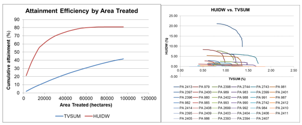
1. Cumulative attainment graphs. These graphs describe results in two ways: 1) how much of a total problem is treated (cumulative attainment of the PCP values), and 2) how much of something is produced (total timber volume, potential building exposure mitigated). Planning areas are ordered by SubunitRank for a specific weighted scenario and effects are summed as a successive number of planning areas are considered. Cumulative attainment graphs are shown for a single weighted scenario (Fig. 6). For instance, Fig. 6 shows attainment in reduction of building exposure; incidental benefits attained in timber volume are also shown, although this output was not prioritized. They can be paneled to produce comparisons between different weighted scenarios. In addition, these graphics can show attainment by ownership, forest, region, and other subcategories.

Tradeoffs or production frontiers

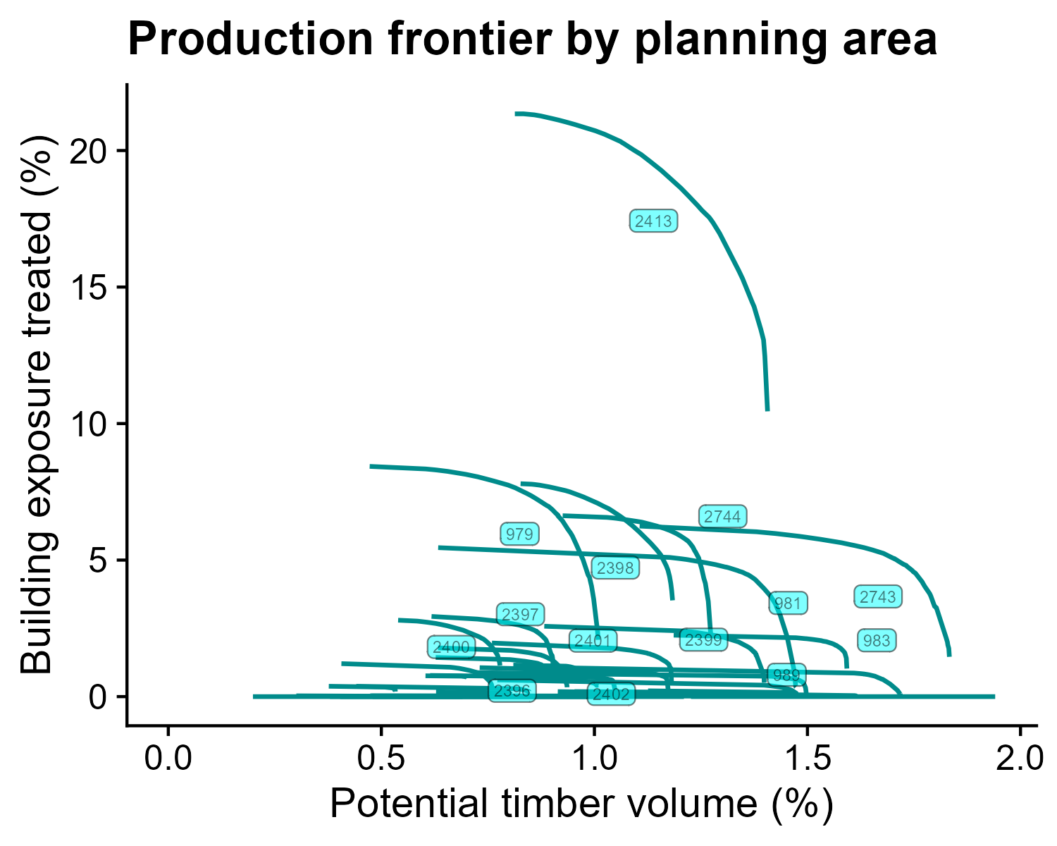
Production frontier (PF) curves are typically grouped at the subunit level, either predefined planning areas or projects output from an optimization run. Each curve graphs the total attainment of two priorities for a given range of weighted scenarios for each single planning area (Fig. 7). In most cases, producing more of one variable will necessarily mean producing less of the other variable. This allows a manager to identify two things: 1) planning areas where both values can be produced at high levels, and 2) solutions for a given planning area where one priority can be increased with a small opportunity cost relative to the other priority. For example, the PF curve for planning area 2413 in Fig. 8 has the highest attainment for both objectives. It is important to understand that each point on a single curve is a different selection of stands within the planning area where one objective is weighted more, less, or equal to the other (as set in the Priorities and Weights panel in Fig. 5). The shorter the curve the fewer combinations of stands are available to increase attainment for a given priority. The longer the curve, the more opportunities there are on the landscape to change a selection of treatment stands to emphasize one metric or another.

2. Production Frontiers. Production frontier (PF) curves are typically grouped at the subunit level, either predefined planning areas or projects output from an optimization run. Each curve graphs the total attainment of two priorities for a given range of weighted scenarios for each single planning area (Fig. 7). Economic principles of scarcity apply to the problem of optimizing treatments for multiple objectives, and thus in nearly all cases, treating to achieve one objective will result in diminished attainment of the other, unless the two are perfectly spatially correlated.  This allows the user to identify: 1) planning areas where both values can be optimized at relatively high levels, and 2) solutions for a given planning area where one priority can be increased with a small opportunity cost relative to the other priority. For example, the PF curve for planning area 2413 in Fig. 8 has the highest attainment for both objectives. It is important to understand that each point on a single curve is a different selection of stands within the planning area where one objective is weighted more, less, or equal to the other (as set in the Priorities and Weights panel in Fig. 5). The shorter the curve the fewer combinations of stands are available to increase attainment for a given priority. The longer the curve, the more opportunities there are on the landscape to change a selection of treatment stands to emphasize one metric or another.

3. Maps. Maps produced within ArcGIS o other software can be used to visualize and sequence planning areas. Mapping requires filtering the results.csv data to a single priority weighting combination (e.g., 0 for timber volume and 1 for structure exposure) and joining the rows from that selection to the project areas shapefile using the Subunit field. The ProjectNum indicates the planning area rank for that scenario ordered by the priority of interest or the weighted value. Maps similar to those shown in Fig. 8 could be created for each weighting combination or scenario. For this example, there were 65 different weighted scenarios, which in turn could produce 65 different maps. Doing so would show how stand selection gradually shifts between the two extremes shown in Fig. 8 under different combinations of weighted priorities. Note also that in this example, some planning areas could not meet the treatment target of 2500 ha, such as those planning areas partially or completely within designated wilderness. These results are noted as ‘Invalid’ in the results output file. A planning area shapefile for the example dataset has been provided (SHF_planarea.shp).  Note that when results for a planning area are invalid the values in the production frontier only represent what ForSysX was able to treat.

6.D. Excel graphing program

As noted in section 6.C there are three primary graphics that are produced using ForSysX outputs, two of these can be created with a custom Excel macro program: cumulative attainment graphs and production frontiers (PFs). The program is designed to take an ForSysX results.csv file as an input and automatically create attainment and PF graphics using a simple dialogue box.

1. Open ForSysOutputGraphs.exe and browse to your ForSysX output results file.  The program automatically searches for fields with “PCP” to populate the Response field section. You should see ETrt_TVSUM_PCP and ETrt_HUIDW_PCP appear (Fig. 9). Note: This graphing program will work without PCP fields. Simply rename fields in the *Results.csv to have PCP in the field names and the program will create attainment and PF graphs for any variables.

2. Make graphing selections. Select both PCP fields so they are highlighted blue. Set the Subset field to <none>, the Planning Area Field should have defaulted to ‘Subunit’ and set the Treated Area Field to ‘TREAT_AREA_HA’ (Fig. 9).

3. Click Create. The program will take a couple of minutes to run and provide progress bar.  Results in Excel will automatically open.

6.E. Optimization Run

The following example application illustrates the spatial optimization capabilities in ForSysX which is the more common application than predefined planning areas and provides more information on the efficiency of alternative scenarios in terms of management objectives and constraints. The spatial optimization algorithm is described in detail in Day et al. (2023).

1. Request ForSysX and the associated archives (See Get Started); see above for ForSys program and Excel graphing program:

   o ForSysX tutorial data for the Shasta-Trinity National Forest study area (ForSysX_Shasta_Tutorial.zip)

   o Note: if you have already run the predefined planning area example above, simply download the xml file instead and use a text editor to change the filename pathways to the location where the shapefile is stored.  Then Load the xml in the ForSys program.

2. Create a folder to store the program and data. Move zip files to that folder and extract their contents to the folder.

3. Open the ForSysX.exe program and select the Load Archive option at the bottom right panel.

4. Navigate to the folder you created above and open STF_opt_example.ltd. The .ltd file is a zipped archive, so ForSysX will ask where you want to put the files. Save the files into the directory of your choice when prompted. This will be your root directory for ForSysX scenario outputs. Your ForSys program should now look like the screenshot in Fig. 11.

5. Interpreting the inputs for the ForSysX optimization scenario: This example analysis from the Shasta-Trinity National Forest identifies ten projects by optimizing building exposure from wildfires ignited on national forest stands that spread to communities. Note that if you hover over any ForSysX setting, popup text will describe the setting. In this analysis, stands available for treatment are set by the Available Field, which in this case describes whether active management is permitted. The Exclude Field removes wilderness, roadless and nationally designated areas from the scenario input. Next, the analysis will look at priority metrics for TVSUM_PCP only; setting the weights and steps as 1 simply identifies that weights are not needed.  Note that here we use the TVSUM_PCP value rather than the SPM. Either metric would work, but since we only have one priority, the range in values is not an issue (see section 1.A.). No treatment thresholds are defined, meaning all manageable stands as defined by the Available Field will be considered. The analysis constrains treatments to 2,500 ha for each of the 20 optimized projects with a 50-ha slack (ForSysX will consider the result valid if it can treat up to 2,450 ha).  No maximum project diameter is specified (-1) and the inverse distance weighting is set at the default value of 0 (see section 1.E.).  The seed stand percent is set at 100 meaning that ForSysX will examine each stand as a seed to build a project.  Reducing this value dramatically reduces the solution time for large landscape. The Effects panel shows that ForSysX will report the following treatment effects: timber volume, percentage timber volume attained, building exposure and percentage building exposure potentially treated (Fig. 11). The suffix STND reflects absolute values while PCP describes the percent of the total produced. ForSysX is set to output both stand csv files and shapefiles of stand selections. Shapefiles can be deselected to speed-up the simulation. A data dictionary for the input shapefile is provided with the tutorial.

6. Run the program (bottom right Run button). If Output Stand Shapefile is selected, the program will take between 2 and 10 minutes to run depending on processor speed.  If Output Stand Shapefile is not selected it will run in a few minutes.

   o Note that all the output files will use the name provided at the top of the ForSysX window, which for this tutorial defaults to SHF_HU_opt_example.

7. The program will provide a progress bar and when completed will allow the user to check the output files for completion.

   o Files generated by ForSys are saved to the directory that you chose when you extracted files from the .ltd archive in step 4.  For a detailed explanation of ForSys outputs, see step 6.B. above.

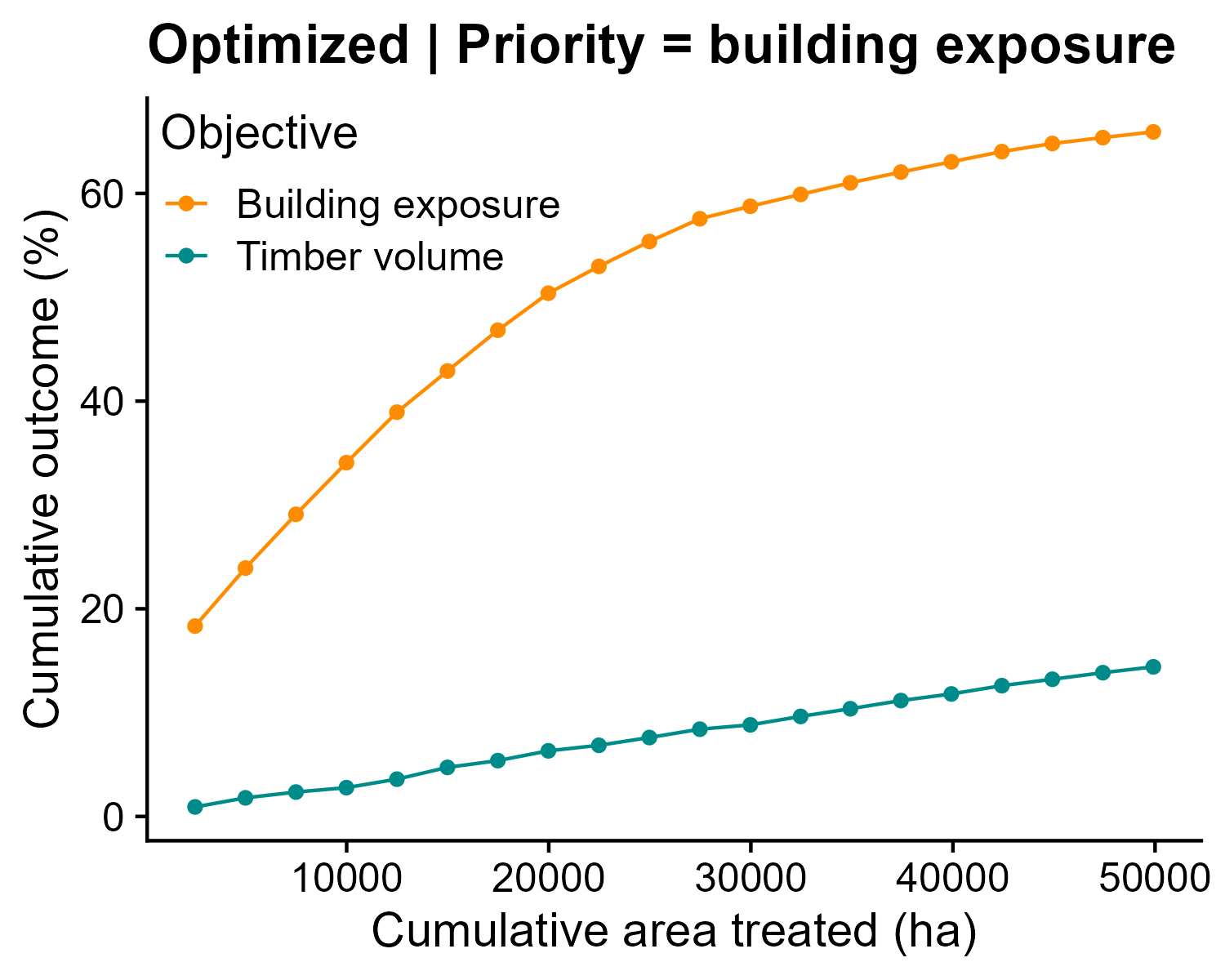
8. Cumulative attainment graph. These graphs describe results in two ways: 1) how much of a total problem is treated (cumulative attainment of the PCP values), and 2) how much of something is produced (total timber volume, potential building exposure mitigated). Projects areas are ordered by ProjectNumber and effects are summed as a successive number of project areas are considered. For instance, Fig. 12 shows attainment in reduction of building exposure; incidental benefits attained in timber volume are also shown, although this output was not included as a priority but rather considered as an effect. In addition, these graphics can show attainment by ownership, forest type, region, and other subcategories.

9. Maps. Maps are produced within ArcGIS (or another mapping program such as QGIS or R), and can be used to visualize and sequence project areas. In this example, the option to output a stand shape file was selected which can be directly imported into a mapping program.  The ProjectNumber indicates the project rank for that scenario and Treat indicates if the stand was or was not treated (1 = treated). In Fig. 13 stands are symbolized based on ProjectNumber where treated (Treat = 1). Note also that in this example, ForSys was able to meet the treatment constraint of 2500 ha. These results are noted as ‘Valid’ in the results output file. Both the treated and untreated stands can also be mapped using the Treat field in the output CSV file and joined to the stand shapefile based on CELL_ID.

Acknowledgments

This tutorial was written by Rachel Houtman, Michelle Day, Fermin Alcasena, and Alan Ager.  Stu Brittain and Alan Ager designed version 1 of ForSysX (formerly the Landscape Treatment Designer).  Ken Bunzel has provided all updates and for version 2 of ForSysX. Thanks to Ana Barros for an external review of this manual, and Cody Evers for testing the tutorial.